Structure

Framework classes

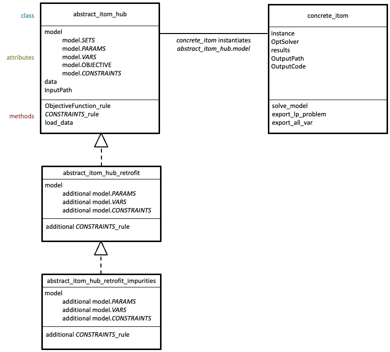
The following inheritance diagrams present the class components of ITOM as implemented in the src/ folder Detailed documentation of the classes, their attributes and methods is available below at the conceptual level and in the components chapter for the concrete implementation.

The class abstract_itom provides the tools to build industry models where every location is directly linked to every other location. The class abstract_itom_hub provides the tools to build industry models where every location in a given region is indirectly linked to every other location in that region through a transport hub. Both classes use objects from the Pyomo library. The class abstract_itom_hub_tinyomo provides the same functionalities as abstract_itom_hub but uses objects from our own tinyomo clone of Pyomo, which allows for larger problems to be modelled through reduced memory consumption.

The abstract classes presented above together with the concrete_itom class form the core of the framework, in three different forms. Each option has its own advantages and disadvantages:

• abstract_itom is adapted to problems with a smaller number of locations where tracking the exchange of products between individual locations is of interest. The number of transport links between locations increases as n*(n-1) with the number n of locations, which can lead to very large problems that cannot be built or solved depending on your hardware.

• abstract_itom_hub is adapted to problems with a larger number of locations where the exchange of products between locations is assumed to happen in a liquid market fashion, i.e. where the transport hub is used to aggregate product flows from all locations in a region and can serve all locations in that region. The number of transport links increases linearily with the number n of locations.

• abstract_itom_hub_tinyomo is adapted to problems becoming too large due to the number of locations, products, and technologies, which results in a very large number of equations that may not fit in memory when the LP problem is built with Pyomo.

The core abstract classes can easily be extended to model more details of industry systems. The subclasses inherit the attributes and methods of the parent class and can define new sets, parameters, variables, constraints, or even objectives. They can also overwrite attributes or methods of the parent class. We have developed the following subclasses available in the src/ folder:

• retrofit: allows for certain production capacities reaching their end-of-life to be retrofitted, that is to be upgraded to a new technology and see its lifetime extended.

• impurities: allows for tracking impurities in input and output products and setting limits on impurity levels in certain products. It can be used, for example, for modelling the production of steel from scrap (or a mix of scrap an iron ore) with several grades of scrap and different impurity tolerances for different steel grades.

All abstract classes are built on the same principles, first defining sets attributes that are used to index the parameters, variables, and constraints attributes that are defined next. Finally, the equations of the LP problem are built as class methods, each being a function referred to as a constraint_rule. This structure is the same whether we use Pyomo or tinyomo to build the LP problem, only the syntax differs.

Class diagram for ITOM

Class diagram for ITOM hub

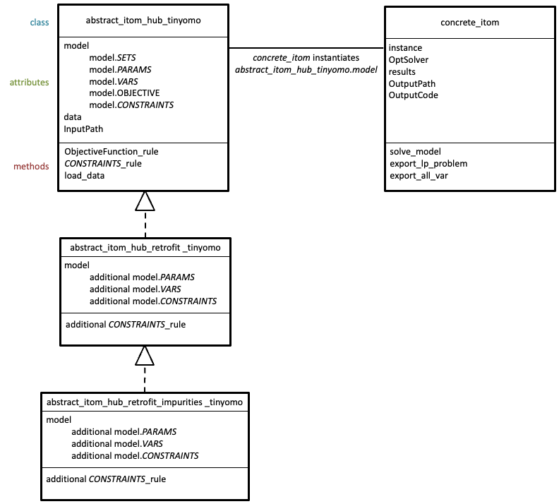
Class diagram for ITOM hub with tinyomo

Basics: sets, parameters, constraints, variables

Building a sectoral model with ITOM (see Sectoral models), data is entered into the model through exogenous parameters. These parameters are indexed with sets (i.e. each parameter is defined for each item in the indexing sets). Equations in the model use exogenous parameters and define or use endogenous variables, also indexed with sets. Every equation in the model is defined as an equality or inequality constraint. See below two examples in pseudo-code to illustrate.

Example 1:

Const. SCA3_TotalAnnualCapacity_1(l,t,y):

      LocalResidualCapacity[l,t,y]
      + LocalAccumulatedNewCapacity[l,t,y]
      = LocalTotalCapacity[l,t,y]

where:

• SCA3_TotalAnnualCapacity_1(l,t,y) is an equality constraint defined for each LOCATION, TECHNOLOGY, and YEAR.

• LocalResidualCapacity[l,t,y] is an exogenous parameter defined for each LOCATION, TECHNOLOGY, and YEAR.

• LocalAccumulatedNewCapacity[l,t,y] is a variable (generated in another constraint) defined for each LOCATION, TECHNOLOGY, and YEAR.

• LocalTotalCapacity[l,t,y] is a variable (generated in this constraint) defined for each LOCATION, TECHNOLOGY, and YEAR.

In plain English, the constraint means that the installed capacity of any given technology in any year and location is the sum of the exogenously provided residual capacity and the endogenously invested new capacity (that has not yet reached its end-of-life).

Example 2:

Const. NCC1_LocalTotalAnnualMaxNewCapacityConstraint(l,t,y):

      LocalNewCapacity[l,t,y]
      <= LocalTotalAnnualMaxCapacityInvestment[l,t,y]

where

• NCC1_LocalTotalAnnualMaxNewCapacityConstraint(l,t,y) is an inequality constraint defined for each LOCATION, TECHNOLOGY, and YEAR.

• LocalNewCapacity[l,t,y] is a variable (generated in another constraint) defined for each LOCATION, TECHNOLOGY, and YEAR.

• LocalTotalAnnualMaxCapacityInvestment[l,t,y] is an exogenous parameter defined for each LOCATION, TECHNOLOGY, and YEAR.

In plain English, the constraint means that the endogenously invested new capacity of any given technology in any year and location cannot exceed exogenously imposed limit for this technology, location, and year.

Sets

Anything modelled with ITOM is either a PRODUCT (e.g. naphta, ethylene, polypropylene, iron ore, raw steel, scrap, klinker, cement), a TECHNOLOGY (e.g. steamcracker, polymerisation plant, blast furnace, kiln) or a TRANSPORTMODE (a particular kind of technology, e.g. pipeline, ship).

The set EMISSION represents a particular kind of products. Other sets relate to the temporal (YEAR) and geographical (REGION, LOCATION) scopes of the model. The last set MODE_OF_OPERATION applies to items defined under TECHNOLOGY.

List of all sets

The following table presents the signification of all input sets defined by the framework and required to build a model.

set	description
YEAR	timeseries of model snapshots
TECHNOLOGY	supply of raw materials (e.g. SUPP_OIL) and industrial production (e.g. STEAMCRACKER)
TRANSPORTMODE	transport of products between locations (e.g. PIPELINE)
PRODUCT	anything that can be used in a technology or transport mode (e.g. NAPHTA, ETHYLENE, H2, ELECTRICITY)
REGION	a geographical system boundary
LOCATION	a production site within a region

Some sets have special requirements for the model to run properly, which are described below.

TECHNOLOGY

As mentioned above, technologies are ubiquitous in the model. Two special types of technologies need to be defined for ITOM-based models to work properly:

1. If you define pipelines (or other point-to-point transport modes) that can run through several locations (i.e. A => B => C => D etc.) you need to list special transfer technologies for each product that can be transported via pipeline. Think of them as pumping stations letting products flow through a location. You could for example name those pipeline_transfert_PRODUCT but any other name would do (see Pipeline transport passing through locations (pipeline_transfert technologies)).

2. If you use the option “transport hub” in your model you need to list special transfer technologies for each product that can be transported between any two locations via the hub. Think of them as dispatch centres routing products through the transport hub. You could for example name those transport_hub_PRODUCT but any other name would do.

LOCATION

If you use the option “transport hub” in your model you need to list a location named TRANSPORT_HUB (name is hardcoded). Any location from any region will be linked to any other location in any region via this hub.

TRANSPORTMODE

Two types of transport modes are expected (they are hardcoded in the framework) and should be listed:

1. ONSITE: allows technologies at any location to exchange products between them within the boundaries of this location (usually at zero or a low cost).

2. OTHER: this is the transport mode that links any location to every other location, either directly or via a transport hub depending on the modelling option selected (hub is the config default).

Parameters

Parameters contain the exogenous data to calibrate a model. They are indexed by the sets presented in the previous section. The following gives a short description and the default value of each exogenous parameter in the framework. Further down, we single out a few parameters that have certain specificities.

Lists of all parameters

The following tables present the data structure and signification of all input parameters defined by the framework and expect data when building a model.

The indices provided below have the following signification: r = REGION, y = YEAR, l = LOCATION, t = TECHNOLOGY, p = PRODUCT, tr = TRANSPORTMODE, m = MODE_OF_OPERATION, e = EMISSION.

Economics

param	index	default	unit	description
DiscountRate	REGION	0.05
DepreciationMethod	REGION	1

Geography

param	index	default	unit	description
Geography	REGION, LOCATION	0	either 1 or 0	Defines in which region R location L is located. 1 defines L ‘is located within’ R. 0 means ‘is not located within’.
TransportRoute	LOCATION, LOCATION, PRODUCT, TRANSPORTMODE, YEAR	0	either 1 or 0	Defines which location L is linked with which location LL in order to enable or disable transport of a specific product with a given transport mode. 1 defines a transport link and 0 ensures that no transport occurs. Values inbetween are not allowed.
TransportCapacity	LOCATION, LOCATION, PRODUCT, TRANSPORTMODE, YEAR	0.0	PJ or Mt / yr	Defines the maximum flow of a given product using a given transport mode between two locations in a given year.

Demand

param	index	default	unit	description
Demand	REGION, PRODUCT, YEAR	0	PJ or Mt	The annual requirement for each output product.

Performance

param	index	default	unit	description
CapacityToActivityUnit	REGION, TECHNOLOGY	1	unit of output (activity) / unit of capacity per year, e.g. PJ/GW-YR, Mt/Mt-YR	For processes whose capacity and activity units are the same, use a factor of 1. If not using yearly time steps, use the length of a time step (e.g. 10 year steps: CapacityToActivityUnit = 10). For power plants we use a factor of 31.536, which is the level of energy production in PJ produced from 1 GW operating for 1 year (1GW * 8760 * 3600 / 10^6).
AvailabilityFactor	REGION, TECHNOLOGY, YEAR	1	fraction of hours in year	Maximum time technology may run for the whole year. Often used to simulate planned outages. The model will choose when to run or not to run.
OperationalLife	REGION, TECHNOLOGY	1	years	Operational lifespan of a process in years.
LocalResidualCapacity	REGION, TECHNOLOGY, YEAR	0	GJ or Mt	The capacity left over from periods prior to the modeling period.
InputActivityRatio	REGION, TECHNOLOGY, PRODUCT, YEAR	0	Ratio	The input (use) of product per unit of activity for each technology (i.e. inverse efficiency).
OutputActivityRatio	REGION, TECHNOLOGY, FUEL, YEAR	0	Ratio	Ratio of output to activity. Should be 1 for a technology/process and its primary output product. Can be different than 1 for a technology/process and its secondary output products.

Technology costs

param	index	default	unit	description
CapitalCost	REGION, TECHNOLOGY, YEAR	0.0	Mio EUR/GJ or Mt Capacity	Total capital cost (including interest paid during construction) per unit of capacity for new capacity additions.
VariableCost	REGION, TECHNOLOGY, YEAR	0.00001	Mio EUR/PJ = EUR/GJ or Mio EUR/Mt	Cost per unit of activity of the technology. This variable records both the O&M costs of processes and costs of each product inputs supplied to those processes.
FixedCost	REGION, TECHNOLOGY, YEAR	0.0	Mio EUR/GJ or Mt of Capacity	The annual cost per unit of capacity of a technology.
TransportCostByMode	REGION, TRANSPORTMODE, YEAR	0.0	Mio EUR/GJ or Mt	Cost of transporting one unit of product.

Capacity constraints

param	index	default	unit	description
CapacityOfOneTechnologyUnit	REGION, TECHNOLOGY, YEAR	0	GJ or Mt	Defines the minimum size of one capacity addition. If set to zero, no mixed integer linear programming (MILP) is used and computational time will decrease.
TotalAnnualMaxCapacity	REGION, TECHNOLOGY, YEAR	99999	GJ or Mt	Maximum total (residual and new) capacity each year.
TotalAnnualMinCapacity	REGION, TECHNOLOGY, YEAR	0	GJ or Mt	Minimum total (residual and new) capacity each year.

Investment constraints

param	index	default	unit	description
LocalTotalAnnualMaxCapacityInvestment	LOCATION, TECHNOLOGY, YEAR	0	GJ or Mt	Maximum new capacity each year. Use this to allow the model investing in existing technologies.
LocalTotalAnnualMinCapacityInvestment	LOCATION, TECHNOLOGY, YEAR	0	GJ or Mt	Minimum new capacity each year. Use this to reflect political or corporate targets.

Activity constraints

param	index	default	unit	description
TotalTechnologyAnnualActivityUpperLimit	REGION, TECHNOLOGY, YEAR	99999	PJ or Mt	Maximum amount of activity that a technology can perform each year.
TotalTechnologyAnnualActivityLowerLimit	REGION, TECHNOLOGY, YEAR	0.0	PJ or Mt	Minimum activity that a technology can perform each year.
TotalTechnologyModelPeriodActivityUpperLimit	REGION, TECHNOLOGY	99999	PJ or Mt	Maximum level of activity by a technology over the whole modelling period.
TotalTechnologyModelPeriodActivityLowerLimit	REGION, TECHNOLOGY	0.0	PJ or Mt	Minimum level of activity by a technology over the whole modelling period.

ResidualCapacity

Technology definitions in this parameter need to be consistent with the definitions implied in the activity and cost parameters. It is up to the analyst to properly document her choices. Concretely a technology can usually be defined with respect to input processing capacity (e.g. Mt naphtha a steam cracker can process in a year) or output production capacity (e.g. Mt ethylene a steam cracker can produce in a year).

Capacities must be provided for the special technologies pipeline_transfert_PRODUCT at the location where pipelines (or other defined point-to-point transport modes) go through. The capacity should be equal to the transport capacity of the transport mode. Think of this transfer technology as a pumping station that can send a product arriving through the pipeline to technologies at the same location that need it and/or forward it further to the next location down the pipeline (see Pipeline transport passing through locations (pipeline_transfert technologies)).

TransportRoute & TransportCapacity

The sheets to fill out in the input Excel file do not have the exact same name as the parameters themselves. The sheets are called TransportRoute_pipeline and TransportCapacity_pipeline, respectively. Those names are hardcoded, so do not change them. The reason is that only specific location to location transport link (e.g. pipelines) should be defined in those sheets.

The following will happen automatically during processing of the input data, before the LP problem is built:

• Each location receives the capability to transport any product ONSITE (that is the name of the transport mode) between technologies installed at the location.

• [If you use the option “transport hub” in your model.] Each location is connected to the transport hub location and the transport hub location is connected to each location with the OTHER transport mode (covers road and rail transport mainly).

• [If you do NOT use the option “transport hub” in your model.] Each location is connected to every other location with the OTHER transport mode.

The transport routes defined in the parameters TransportRoute_pipeline and TransportCapacity_pipeline are directional. The two REGION columns in the input dataset mean “region from” and “region to”, respectively in that order. Therefore, bi-directional routes (e.g. a pipeline between two locations that exchange the same product both ways depending on the availability of production capacity at both ends of the pipeline) should be defined *with the same capacity* both ways.

Transport routes that use a multi-purpose transport mode must be defined in both parameters for each product that can be transported with this one transport mode, *with the same capacity* for each product representing the overall capacity of the transport link.

InputActivityRatio & OutputActivityRatio

These two parameters have to be consistent with one another and with how capacity of a given technology is defined (in general and in particular in parameter ResidualCapacity), concretely whether it is defined with respect to input processing capacity (e.g. Mt naphtha a steam cracker can process in a year) or output production capacity (e.g. Mt ethylene a steam cracker can produce in a year).

The special technologies pipeline_transfert_PRODUCT and transport_hub_PRODUCT must be defined with InputActivityRatio = OutputActivityRatio = 1.

CapitalCost, VariableCost & FixedCost

Technology definitions in these parameters have to be consistent with the capacity and activity parameters. The cost parameters are defined for each technology at the regional level. These costs can change over time, e.g. assuming declining costs due to accumulated learning.

Note

Variable costs are defined at the regional level, to keep data input simpler

and save some mode equations. However, variable costs defined at the local level

would allow for a higher granularity of production costs. A typical example is different

process energy costs (e.g. as electricity, heat, hydrogen) for different locations within the same region.

See Local energy prices for more information on how to deal with such a case.

The special technologies pipeline_transfert_PRODUCT must be defined with very high capital cost so that they are not installed in locations where they were not explicitly placed as ResidualCapacity. The special technologies transport_hub_PRODUCT must not be defined, they will receive CapitalCost = 0 by default and be installed in transport hubs only.

TimeStep

An item in the set YEAR can be understood as a label for a time period of length TimeStep. For mainly practical reasons (server memory and processing capacities) we do not run the model with a yearly resolution but for time periods of length 10 (we hope to be able to reduce this length to 5). Note that 10 | Wuppertal InstituteEDM-invest TimeStep is required for each “year” (i.e. each item in set YEAR) but the same value is expected for each.

MatchTechnologyRetrofit

The two TECHNOLOGY columns in the input dataset mean “technology that can be retrofitted” and “retrofit technology”, respectively in that order. A retrofit technology can also be a technology that can be retrofitted (again). In such a case, the same technology name appears in both columns.

Constraints

The complete list of constraints (i.e. equations in the framework) is available in the components chapter.

Core constraints of the model define product flows in the system. There are two categories of flows: production and use of products by technologies.

Production

The production (or output) of a product from a technology at a given location in a given mode of operation is equal to the (rate of) activity of this technology multiplied with a product output to production activity ratio entered by the analyst (parameter OutputActivityRatio):

Production = Activity * OutputActivityRatio

Use

The use (or input) of a product by a technology at a given location in a given mode of operation is equal to the (rate of) activity multiplied with a product input to production activity ratio entered by the analyst (parameter InputActivityRatio):

Use = Activity * InputActivityRatio

Both constraint categories above require the definition of core constraints pertaining to the activity of technologies.

Activity

The activity of a given technology at a given location is decided by the solver in order to generate production to meet demand:

Activity <= Capacity * AvailabilityFactor * CapacityToActivityUnit

There are several additional constraints that can be put on the activity level (minimum and maximum activity). These are defined at the regional level (i.e. they regard the sum of activities in the locations of a region) and can apply either annually (parameters TotalTechnologyAnnualActivityUpperLimit and TotalTechnologyAnnualActivityLowerLimit) or over the whole modelling period (parameters TotalTechnologyModelPeriodActivityUpperLimit and TotalTechnologyModelPeriodActivityLowerLimit).

The next core constraint category builds on the above, ensures that demand is met, and product flows balanced.

Product balance

For each year and region, the total production of each product + imports of this product from locations outside the region should be larger than or equal to this product’s demand in the considered region. If production + imports is larger than demand, this can mean that this region is a net exporter (via transport to locations outside the region):

Production + Import - Export >= Demand

Note

The Demand parameter passed to the model represents the final net demand for a

product (in our case an end-product such as a polymer), i.e. it does not account for potential

intermediary product use in the industry.

As consequence the shadow prices from this constraint give no insight into the marginal production

costs of intermediates. It is, however, possible to work around this limitation and access this information (see Tracking shadow prices of intermediate and final products).

All the above constraints rely at some level on the constraints dealing with capacity presented below.

New capacity

For each technology, constraints on minimum and maximum investments per time step are defined locally. This allows to reflect business and political decisions known today that will affect investments in the future, or simply to simulate the impact of potential such decisions. The corresponding parameters are LocalTotalAnnualMaxCapacityInvestment and LocalTotalAnnualMinCapacityInvestment.

Installed capacity

For each year the available installed capacity is equal to the sum of the exogenously given residual capacity, the accumulated new capacity decided by the solver for the previous time steps (that has not reached its end-of-life yet) and the retrofitted capacities:

Installed capacity = Residual capacity
                     + SUM past New capacity
                     + Retrofits

Both upper and lower limits can be set for the total installed capacity at the regional level. This may be used to reflect political targets set e.g. by countries . The corresponding parameters are TotalAnnualMaxCapacity and TotalAnnualMinCapacity.

The framework can include or exclude retrofitting (default is include) of production capacities reaching their technical end-of-life. Retrofitting rules obey to their own set of constraints.

Retrofitting

The parameter MatchTechnologyRetrofit defines which technologies can be retrofitted with which retrofit technologies. The model checks at each time step (except in the first one, where retrofitting cannot happen) which capacity of “technologies that can be retrofitted” reached end-of-life and might therefore indeed be retrofitted. There are two cases:

1. The exogenously provided residual capacity of a technology “that can be retrofitted” decreases between two time steps: this delta capacity is a potential for retrofit.

2. The endogenously installed new capacity of a technology “that can be retrofitted” reaches its end-of-life: this capacity is a potential for retrofit.

Investment in new retrofit technology capacity is then constrained as maximum 110% of the potential for retrofit (the 1.1 factor is hardcoded):

SUM Retrofits <= 1.1 * Capacity reaching EOL

Another core feature of the framework is the capability to exchange products between locations, as defined in the constraints presented next.

Transport

Exchange capabilities are defined with directional transport links (parameter TransportRoute) between locations (regardless of the regions these locations belong to). Between two locations there can exist no transport link or one or more links, each using a different mode of transport (defined in the Set TRANSPORTMODE). For each transport link between two locations, a maximum yearly carrying capacity is provided (parameter TransportCapacity).

Transport flows must then comply with a number of constraints.

Transport capacity

For each product, each transport mode, each year, transport from location L1 to location L2 is either smaller or equal to the transport link capacity if a transport route exists, or 0 if there is no route. If the route is bi-directional the sum of transport from L1 to L2 and L2 to L1 is smaller or equal to the transport link capacity in one direction (capacity of both directions should be equal). If the transport mode is multi-purpose (i.e. can transport different products in separate batches) the sum of the quantities transported for all products is smaller or equal to the transport capacity:

SUM_products ( Transport L1 to L2 + Transport L2 to L1 ) <= Transport capacity

Outgoing & Incoming transport

At each location L the total quantity of each product transported to all other locations each year is smaller or equal to the production of this product at location L. This deals with locations at the end of the value chain (that generate end-products that are neither used by any technology nor need to be transported, when assuming that locations produce for their own regional demand). It also covers locations with multi-output technologies that have to run to produce a minor by-product thus generating a surplus of a major output:

SUM_locations Transport[product] L0 to L <= Production[product] in L0

At each location L the total quantity of each product transported (arriving) from all other locations each year is equal to the use of this product at location L:

SUM_locations Transport[product] L to L0 = Use[product] in L0

Import & Export

Import and export refer to product flows between regions while transport refers to product flows between locations. Imports to a region R are the sum of the transport flows from locations outside that region R to locations in that region R. Exports from a region R are the sum of the transport flows from locations in that region R to locations outside that region R.

Transport Hubs

Hubs are a special kind of location that must be listed in the Set Hublocation. Only a special kind of technology (that must be listed in the Set HubTechnology) can be installed at a transport hub. Think of those technologies as switch stands that redirect transport flows from one location to another through the hub. No product is consumed in a hub, all product flows arriving at the hub are forwarded by the hub technologies (therefore use = production) and exit the hub:

SUM_locations Transport[product] L to Hub
    = Use[product] in Hub
    = Production[product] in Hub
    = SUM_locations Transport[product] Hub to L

Last but not least the constraints related to costs presented below make up their own category of core constraints.

Investment Costs, Operational Costs & Emission Costs

Investment costs are accounted for in full on the year new capacity is commissioned. Operational costs consist of yearly variable costs depending on activity levels and yearly fixed costs depending on installed capacity. Emission related costs depend on activity levels, emission intensities and emission penalties (e.g. CO₂ prices):

Investment cost = New capacity * CapitalCost
Operational cost = Activity * VariableCost + Capacity * FixedCost
Emission cost = Activity * EmissionActivityRatio * EmissionPenalty

Transport Costs

Transport cost intensities for each mode of transport (parameter TransportCostByMode) are defined regionally (and can vary over time, e.g. if assuming that shipping costs will increase). Actual transport costs, however, are first calculated at the local level (as model variables). For each location, transport costs for a given product are the costs of transporting this product FROM other locations to that location (as the sum of the quantities transported per mode of transport multiplied by the specific costs of each mode of transport). In other words, the importer is the buyer and pays the transport costs.

When aggregated at the regional level, transport costs include both intra-regional transport and imports from other regions. There is no double-counting, however, since transport costs are only registered at the importing location.

Salvage Value

Howells et al. (2011)[1] describe the implementation of salvage value in OSeMOSYSas follows:

“When a technology is invested in during the model period but ends its operational life before, it is assumed to have no value at the end of the model period. However, if a technology (invested in during the model period) still has some component of its operational life at the end of the period, that should be estimated. Several methods exist to determine the extent to which a technology has depreciated. And this in turn is used to calculate its salvage value by the end of the period. […] A salvage value is determined, based on the technology’s operational life, its year of investment and discount rate. Following this it is discounted to the beginning first model year by a discount rate applied over the modelling period.”

The type of depreciation used to calculate the salvage value is determined in the parameter DepreciationMethod:

• 1: Sinking fund depreciation (default)

• 2: Straight line depreciation

Discounted costs

Each cost item [capital, fixed, variable, transport, salvage value, emission penalties] should be calculated in constant monetary terms and then discounted to determine a net present value (NPV). Since in our model we calculate costs first at the local level and then aggregate at the regional level, we try to discount costs early, i.e. already at the local level, so as to allow comparisons of different cost categories across both locations and time.

Variable names give indications on the level processing of different cost items, for example:

• LocalCapitalInvestment: local, undiscounted

• LocalDiscountedCapitalInvestment: local, discounted

• DiscountedCapitalInvestment: regional, discounted

Footnotes

[1]

Howells, M., Rogner, H., Strachan, N., Heaps, C., Huntington, H., Kypreos, S., Hughes, A., Silveira, S., DeCarolis, J., Bazillian, M., Roehrl, A. (2011) OSeMOSYS: The Open Source Energy Modeling System - An introduction to its ethos, structure and development. Energy Policy, 39 (2011), 5850–5870.